Definition: an inner product space in which each Cauchy sequence of vectors has a limit.
Sounds daunting, however, in quantum computing we only care about finite dimensional space. In this case a Hilbert space degenerates to exactly a “normal” inner product space, which is what we learned in our undergraduate level linear algebra course.
Conjugate transpose of \(x\) (which is a row vector): \(x^{\dagger}\)
Inner product of \(x\) and \(y\): \(x^{\dagger}y\) or \(\braket{x}{y}\)
A reminder: Doing a inner product in complex vector space requires taking a “conjugate transpose” instead of simply a “transpose”.
In quantum computing, people usually use a different notation to represent vectors:
Column vector: \(\ket{\varphi}\)
Conjugate transpose of \(\ket{\varphi}\) (which is a row vector): \(\bra{\varphi}\)
Inner product of \(\ket{\varphi}\) and \(\ket{\psi}\): \(\braket{\varphi}{\psi}\)
The advantage of Dirac notation is that we can easily know whether a value is a column vector, a row vector, or a scalar. Read the article by Prof. E. F. Redish for more information.
Most literature only introduces this kind of measurements.
Observable \(M = \sum_m m P_m\), a Hermitian operator. \(P_m\) is a orthogonal projection matrix, i.e., \(P^2 = P^{\dagger} = P\).
In quantum mechanics, the measurement of an observable \(M\) prepares an eigenstate of \(M\), and the observer learns the value of the corresponding eigenvalue.
“Measure in basis \(\ket{m}\)” means \(P_m = \ket{m}\bra{m}\). Often people simply list a set of basis instead of giving the observable \(M\).
For state \(\ket{\psi} = \sum_{i,j} \alpha_{i,j} \ket{u_i}\ket{v_j}\), where \(\ket{u_i}\), \(\ket{v_j}\) are orthonormal bases. We only measure the first qubit using observable \(M=\sum_{m} m P_m\). Since the projection only applies on the first qubit, the operator we use is actually \(P_m \otimes I = \ket{m}\bra{m} \otimes I\).
The trace of an operator \(A\) is defined as the sum of its diagonal entries:
\[\tr(A) = \sum_{i} \bra{i}A\ket{i}\]
The trace is the same no matter which basis you use, so it is a property of the operator, not of the basis you choose.
For a composite system \(AB\), let \(\ket{a}\) and \(\ket{b}\) be basis sets for \(A\) and \(B\), for an operator \(O=O_A \otimes O_B\), the trace of \(O\) is:
\[\begin{split}
\tr(O) &= \sum_{a,b}\bra{a,b}O\ket{a,b}\\
&= \sum_{a,b} (\bra{a} \otimes \bra{b})(O_A\otimes O_B)(\ket{a}\otimes\ket{b})\\
&= \sum_{a,b} \bra{a}O_A\ket{a} \bra{b}O_B\ket{b}\\
&= \sum_a \bra{a}O_A\ket{a} \sum_{b} \bra{b}O_B\ket{b}
\end{split}
\]
The result is simply the product of traces of \(O_A\) and \(O_B\) in their respective Hilbert spaces, i.e.,
\[\tr(A\otimes B) = \tr(A)\tr(B)\]
Similar to the trace, a partial trace is an operator that only traces over a part of the system. For example, if we “trace over B”, we eliminate the variables pertaining to B and what we get is an operator acting only on the Hilbert space of A.
\[\begin{split}
\tr_B(O_A\otimes O_B)
&= \sum_b (I_A \otimes \bra{b})(O_A\otimes O_B)(I_A\otimes\ket{b})\\
&= \sum_b O_A \bra{b}O_B\ket{b}\\
&= \tr(O_B)O_A
\end{split}
\]
More formally, we can define partial trace as follows (from the lecture notes by Dave Bacon):
\[\tr_B(\rho) = \sum_{i=1}^{\dim \mathcal{H}_{B}} \bra{\phi_i}_B \rho \ket{\phi_i}_B\]
where the quantum system is defined in Hilbert space \(\mathcal{H}=\mathcal{H}_A \otimes \mathcal{H}_B\), and \(\ket{\phi_i}\) is a basis for \(\mathcal{H}_B\). \(\ket{\phi_i}_B \triangleq I_A \otimes \ket{\phi_i}\). Note that many literature simply omits the identity \(I_A\), which is a bit confusing.
Another definition in Nielsen & Chuang, which is not very intuitive in my opinion:
Suppose we have physical systems A and B, whose state is described by a density
operator \(\rho^{AB}\). The reduced density operator for system A is defined by:
\[\rho^A \triangleq \tr_B(\rho^{AB})\]
A quantum operation is just a linear map that maps density matrices to density matrices:
\[\rho’ = \mathcal{E}(\rho)\]
It is a general tool for describing the evolution of quantum systems, for example, unitary transformations and measurements are all quantum operations.
Two equivalent representation of quantum operators:
Suppose we have a system in state \(\rho\), which is sent into a box which is coupled to an environment with state \(\rho_{\text{env}}\). After the box’s transformation \(U\) the system no longer interacts with the environment, and thus we perform a partial trace over the environment to obtain the reduced state of the system alone:
\[\mathcal{E}(\rho)=\tr_{\text{env}} \left[ U(\rho \otimes \rho_{\text{env}}) U^{\dagger}\right]\]
Another way of representing quantum operations is called the Operator-Sum Representation:
\[\mathcal{E}(\rho)=\sum_k E_k \rho E_k^{\dagger} \quad \text{with } \sum_k E_k^{\dagger}E_k=I\]
The operators \(\set{E_k}\) are known as operation elements or Kraus operators for the quantum operation \(\mathcal{E}\).
The derivation of equivalence between the two representations, i.e., Equation (8.10) in the textbook by Nielsen & Chuang is not trivial:
Given a superposition of address in the address register \(a\), QRAM returns a superposition of data in the data register \(d\), correlated to the address register. Let \(D_i\) be the content of the \(i\)th memory cell. This is shown in the formula:
\[\sum_{i} \alpha_i \ket{i}_a \longrightarrow \sum_{i} \alpha_i \ket{i}_a \ket{D_i}_d\]
7.1 Pauli Group over \(n\) Qubits: \(\mathcal{P}_n\) #
\(\mathcal{P}_1\) on 1 qubit has 16 elements (2×2 unitary matrices) consisting of all the Pauli matrices:
\[I=\begin{bmatrix}1&0\\0&1\end{bmatrix}, \quad X=\begin{bmatrix}0&1\\1&0\end{bmatrix}, \quad Y=\begin{bmatrix}0&-i\\i&0\end{bmatrix}, \quad Z=\begin{bmatrix}1&0\\0&-1\end{bmatrix}\]
together with the products of these matrices with factors \(\pm 1\) and \(\pm i\).
\(\mathcal{P}_n\) is generated by the operators described above applied to each of \(n\) qubits in the tensor product Hilbert space \((\CC^2)^{\otimes n}\).
Note
\(X\) gate is like a “NOT” gate, \(\ket{0} \mapsto \ket{1}\) and \(\ket{1} \mapsto \ket{0}\).
\(Z\) gate multiplies -1 if input is \(\ket{1}\).
\(Y\) gate \(\ket{0}\mapsto i\ket{1}\), and \(\ket{1}\mapsto -i\ket{0}\).
7.2 Clifford Group over \(n\) Qubits: \(\mathcal{C}_n\) #
The Clifford group is defined as the group of unitaries that transforms Paulis into other Paulis:
\[\mathcal{C}_n = \set{V \in U(2^n): V P V^{\dagger} \in \mathcal{P}_n, \forall P \in \mathcal{P}_n}\]
Given two density matrix \(\rho\) and \(\sigma\), the fidelity is generally defined as the quantity
\[F(\rho, \sigma) = \left(\operatorname{tr} \sqrt{\sqrt\rho \sigma\sqrt\rho}\right)^2\]
Note that for a pure state \(\ket{\psi}\), the square root of its density matrix is the density matrix itself (easy to verify).
Usually we compute the fidelity between a pure state \(\ket{\psi}\) and an arbitrary mixed state \(\rho\).
The average fidelity of a quantum channel \(\mathcal{E}\) is defined by
\[F(\mathcal{E})=\int \dd{\psi} \bra{\psi} \mathcal{E}(\ket{\psi}\bra{\psi})\ket{\psi}\]
where the integral is over the uniform (Haar) measure on state space, normalized so \(\int \dd{\psi}=1\).
Where \(\text{XOR}_s(x)\) is defined as XOR of bits \(x_i\) where \(s_i=1\). I.e., \(\text{XOR}_s(x)=\left(\sum_{i: s_i=1}^n x_i\right) \mod 2 = \left(\sum_{i=1}^n s_ix_i\right) \mod 2\).
Denote \(\ket{g} \triangleq \frac{1}{\sqrt{N}} \sum_{x=0}^{N-1} g(x) \ket{x}\), where \(g: \{0,1\}^n \to \CC\) and satisfies \(\frac{1}{N} \sum_{x=0}^{N-1} |g(x)|^2=1\) (so \(\ket{g}\) is really a quantum state).
Define \(\mathcal{X}_s(x) \triangleq (-1)^{s \cdot x}\), then the above equation can be written as
\[H^{\otimes n} \ket{s} = \ket{\mathcal{X}_{s}}\]
Note that \(H^{\otimes n}\) is its own inverse, so we also have
\[H^{\otimes n} \ket{\mathcal{X}_{s}} = \ket{s}\]
Using this transform, we can get some useful results:
\(\ket{\mathcal{X}_0}, \ket{\mathcal{X}_2}, \dots, \ket{\mathcal{X}_{N-1}}\) are orthonormal.
Notation (Important)
The conventions for the name of “QFT” and “inverse QFT” vary. This is sometimes annoying because Nielsen & Chuang uses notations where QFT has the same effect as the classical inverse Discrete Fourier Transform (DFT), see here for details.
So in the following we will only use \(\text{DFT}\) instead of \(\text{QFT}\). Note that \(\text{DFT}\) means inverse QFT, and \(\text{DFT}^{\dagger}\) means QFT if you follow Nielsen & Chuang’s notation.
Therefore if \(\ket{x}\) is a basis state, i.e., it is a vector where only the \(x\)-th entry is 1 (index starting with 0), we have the inverse Quantum Fourier Transform:
After Alice measures the first two qubits in Bell basis, she will get one of the Bell states, and depending on the outcome, she can send two classical bits to instruct Bob to recover the state \(\ket{\psi}\).
Suppose we have a one-qubit unitary \(U\) which has an eigenvector \(\ket{\psi}\) and \(e^{2\pi i \theta}\) is the corresponding eigenvalue.
Start with \(\ket{0}\ket{\psi}\), apply the Hadamard gate on the first qubit and then the controlled-\(U\) gate (denoted by \(C(U)\)) on the two qubits (the first qubit is the control bit), we have
\(S_0\) changes the sign of the amplitude if and only if the state is \(\ket{0}\). The algebraic expression is \(S_0 = I-2\ket{0}\bra{0}\). In other words, \(-S_0\) is just the sign-implementation of the logical OR function: \(Q^{\pm}_{\text{OR}}\).
\(S_{\chi}\) changes the sign of the amplitudes of the “good” states:
\[S_{\chi}\ket{x} = \left\{
\begin{array}{l@{\quad:\quad}l}
-\ket{x} & \text{if } \chi(x)=1\\
\phantom{-}\ket{x} & \text{if } \chi(x)=0
\end{array}\right.
\]
The algebraic expression is \(S_{\chi} = I-2\Pi_1\), where \(\Pi_i\) is a projection operator defined as
\[\Pi_i=\sum_{x: \chi(x)=i} \ket{x}\bra{x}, \quad i \in \set{0,1}\]
Intuitively, \(\Pi_0\) maintains all the “bad” states and maps all the “good” states to 0. \(\Pi_1\) maintains all the “good” states and maps all the “bad” states to 0. In particular, if there is only one “good state”, say \(\ket{\psi}\), then \(S_{\chi} = I-2\ket{\psi}\bra{\psi}\).
Let \(\mathcal{A}\) be any quantum algorithm (unitary) such that \(\mathcal{A}\ket{0} = \sum_{x} \alpha_x \ket{x}\), and we say the algorithm is “successful” if a “good” result is produced when \(\mathcal{A}\ket{0}\) is measured. Define
We call \(\ket{\Psi}\) the “initial state” because it will be used as the input state of the whole algorithm. Intuitively, \(\ket{\Psi_0}\) is a superposition of all the “bad” states, \(\ket{\Psi_1}\) is a superposition of all the “good” states. Note that \(\ket{\Psi_i}\) are orthogonal. Here we also abuse the notation because \(\ket{\Psi_i}\) are NOT normalized. By definition, we have \(\ket{\Psi} = \ket{\Psi_0}+\ket{\Psi_1}\), and \(S_{\chi}\ket{\Psi_0}=\ket{\Psi_0}\), \(S_{\chi}\ket{\Psi_1}=-\ket{\Psi_1}\).
In fact, \(a\) is the success probability of algorithm \(\mathcal{A}\), i.e., the probability of getting a “good” state by directly measuring \(\mathcal{A}\ket{0}\).
Define the angle \(0<\theta\leq \frac{\pi}{2}\) such that \(\sin^2(\theta) = a\). And we normalize \(\ket{\Psi_1}\) and \(\ket{\Psi_0}\) to \(\frac{1}{\sqrt{a}}\ket{\Psi_1}\) and \(\frac{1}{\sqrt{1-a}}\ket{\Psi_0}\) respectively, so that they can be used as an orthonormal basis. We call the space spanned by them \(\mathcal{H}_{\Psi}\). The above lemma can be reformulated as:
Thus if a vector is in the space \(\mathcal{H}_{\Psi}\), applying \(Q\) on it corresponds to a rotation by the angle \(2\theta\), which can be represented by the rotation matrix:
Now measure, the probability of finding a “good” state is \(\sin^2((2n+1)\theta)\). To maximize it, let \((2n+1)\theta=\frac{\pi}{2}\), we get \(n=\frac{\pi}{4\theta}-\frac{1}{2}\). So we choose \(n=\lfloor \frac{\pi}{4\theta}\rfloor\). In this case, we have:
I.e., by applying \(Q\) for \(\Theta\left(\frac{1}{\sqrt{a}}\right)\) times, we can find a “good” state with high probability.
Since the algorithm \(\mathcal{A}\) has a success probability \(a\), in classical case, to find a “good” output, the expected number of applications of \(\mathcal{A}\) is \(\frac{1}{a}\). Therefore we obtain a quadratic speedup over the best possible classical algorithm.
Note that this algorithm requires that the value of \(a\) is known so that \(n\), the number of times we apply \(Q\), can be computed.
Geometric Illustration
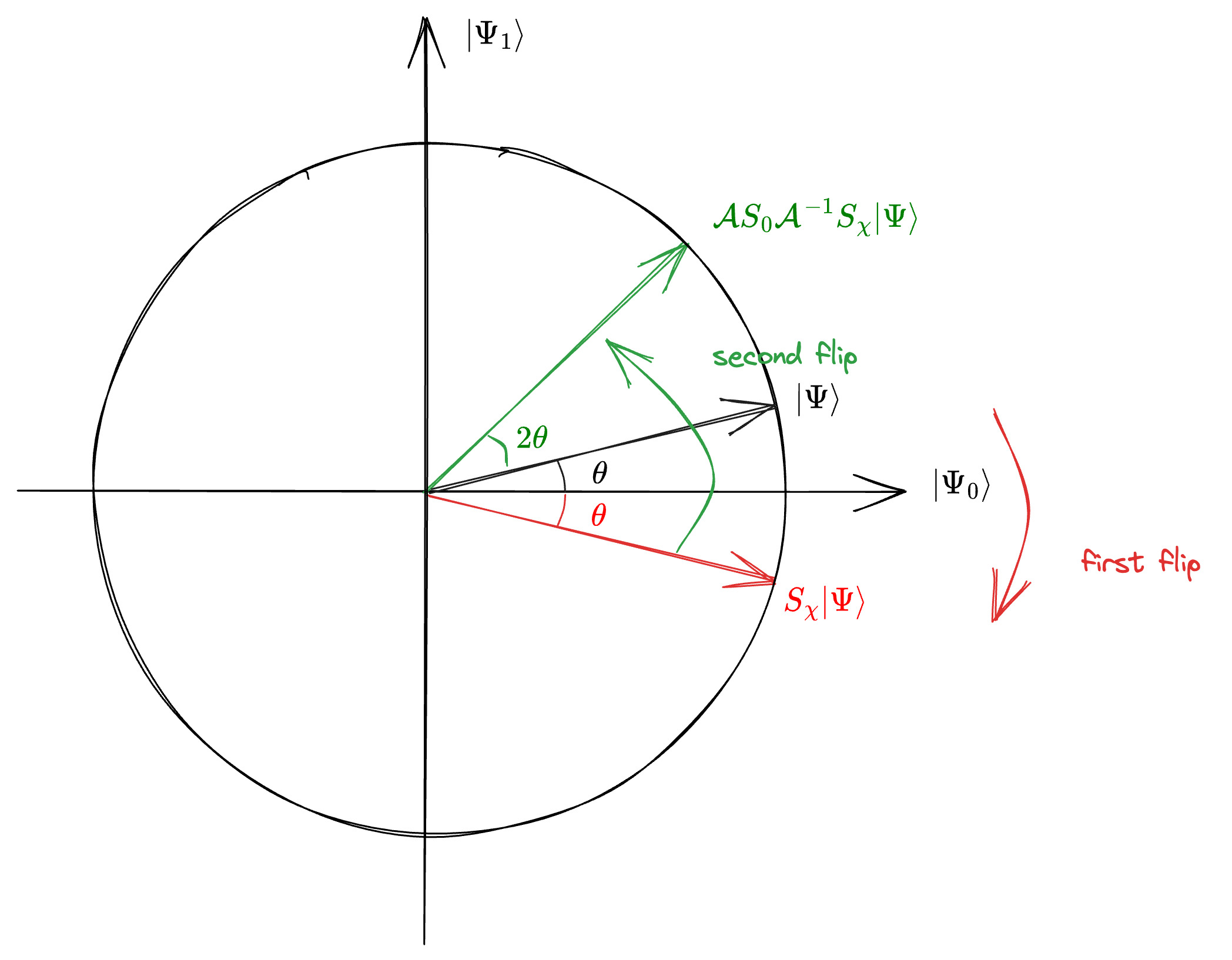
When applying operator \(Q=-\mathcal{A}S_0\mathcal{A}^{-1}S_{\chi}\) to the initial state \(\ket{\Psi}\), the operation can be regarded as two flips, as shown in the figure:
Figure 1: Geometric Illustration of Amplitude Amplification (image credit: mm)
(Shown in red) First apply \(S_{\chi} = I-2\Pi_1\), which geometrically flips a vector with respect to \(\ket{\Psi_0}\), the superposition of all the “bad” states.
(Shown in green) Then apply \(-\mathcal{A}S_0\mathcal{A}^{-1} = -I + 2 \ket{\Psi}\bra{\Psi}\), which geometrically flips a vector with respect to \(\ket{\Psi}\), the initial input state.
The overall effect is to rotate the initial state towards \(\ket{\Psi_{1}}\), the superposition of “good” states, by an angle of \(2\theta\) (This is a general conclusion, A rotation equals two reflections). The amplitude amplification algorithm essentially repeats this procedure \(n\) times, then measure.
Given a Boolean function \(f: \set{0,1, \dots, N-1} \to \set{0,1}\) satisfying that there exists a unique \(x_0\) on which \(f\) takes value 1, and Grover’s algorithm is to find \(x_0\).
Grover’s algorithm is a spacial case of the Amplitude Amplification algorithm. let \(\chi=f\), and let \(\mathcal{A}=H^{\otimes n}\) be the Hadamard transform on \(n\) qubits. The operator
\[Q = -\mathcal{A}S_0\mathcal{A}^{-1}S_{\chi} = -H^{\otimes n}S_0 \left(H^{\otimes n}\right)^{\dagger}S_f = H^{\otimes n} Q^{\pm}_{\text{OR}} H^{\otimes n}S_f\]
This algorithm finds \(x_0\) with high probability by using \(O(\sqrt{N})\) evaluations of function \(f\).
Given a unitary operator \(U\), which has an eigenvector \(\ket{\psi}\) with eigenvalue \(e^{2\pi i\theta}\), \(0\leq\theta<1\). We assume that \(\ket{\psi}\) is known and \(\theta\) is unknown. The goal of the algorithm is to estimate \(\theta\).
Intuition: Using Phase Kickback to write the phase of \(U\) (in the Fourier basis) to \(t\) qubits in the “counting register”. Then using the inverse transform to translate this from the Fourier basis into the computational basis, which we can measure. \(t\) is chosen according to the accuracy we wish to have in our estimate of \(\theta\).
Prepare state. The first register (“counting register”) has \(t\) qubits initialized to \(\ket{0}\). The second register is initialized to \(\ket{\psi}\):
\[\ket{\psi_0}=\ket{0}^{\otimes t} \ket{\psi}\]
Apply \(H^{\otimes t}\) on the first register:
\[\ket{\psi_1}= \frac{1}{\sqrt{2^t}} \left( \ket{0}+\ket{1} \right)^{\otimes t} \ket{\psi} \]
Apply controlled-\(U^{2^j}\) on the second register with \(0\leq j \leq t-1\), where the control bit is the \(j\)-th qubit in the first register, respectively. (See Figure 5.2 in Nielsen & Chuang)
\(U^{2^j}\) is defined as:
\[U^{2^j} \ket{\psi} = U^{2^j-1}U\ket{\psi} = U^{2^j-1} e^{2\pi i \theta}\ket{\psi} = \dots = e^{2\pi i 2^j \theta}\ket{\psi}\]
Using the property of phase kickback:
\[C(U^{2^j})(\ket{+}\ket{\psi}) = \frac{1}{\sqrt{2}} C(U^{2^j})\left( \ket{0}\ket{\psi} + \ket{1}\ket{\psi} \right) = \frac{1}{\sqrt{2}} \left( \ket{0} + e^{2\pi i 2^j \theta} \ket{1} \right) \otimes \ket{\psi} 1\]
We get the final state of the both registers:
\[\begin{split}
\ket{\psi_2} &= \frac{1}{\sqrt{2^t}}\left( \ket{0} + e^{2\pi i 2^{t-1} \theta} \ket{1} \right) \otimes \dots \otimes \left( \ket{0} + e^{2\pi i 2^1 \theta} \ket{1} \right) \otimes \left( \ket{0} + e^{2\pi i 2^0 \theta} \ket{1} \right) \otimes \ket{\psi}\\
&= \frac{1}{\sqrt{2^t}} \sum_{k=0}^{2^{t}-1} e^{2\pi i k \theta} \ket{k}\ket{\psi}\\
&= \left(\text{DFT}^{\dagger}_{2^t} \ket{2^t \theta}\right) \otimes \ket{\psi} \quad \text{(if } 2^t\theta \text{ is an integer)} \end{split}
\]
The second equality is due to the definition of the Quantum Fourier Transform.
Perform \(\text{DFT}_{2^t}\) on the first register, if \(2^t\theta\) is an integer, we get
\[\ket{2^t \theta}\ket{\psi}\]
Now measure and we get the outcome \(2^t\theta\) in the first register, so we know \(\theta\).
If \(2^t\theta\) is not an integer, we can approximate \(\theta\) by rounding \(2^t\theta\) to the nearest integer, see discussion below.
Performance:
In summary, exactly \(\sum_{j=0}^{t-1} 2^j = 2^t-1\) controlled-\(U\) gates are used.
If \(2^t\theta\) is an integer, then we can get \(\theta\) exactly with probability 1.
If \(2^t\theta\) is not an integer, we round it to the nearest integer \(a\), i.e.,
\[2^t\theta = a + 2^t\delta\]
where \(-\frac{1}{2}\leq 2^t\delta \leq \frac{1}{2}\), the \(2^t\) factor is only for the convenience of the following derivation.
We will prove that when measuring the first register, we get outcome \(a\) with high probability.
Proof
At step 4, applying \(\text{DFT}_{2^t}\) on the first register, which has state:
\[\frac{1}{\sqrt{2^t}} \sum_{k=0}^{2^{t}-1} e^{2\pi i k \theta} \ket{k}\]
We get:
\[\begin{split}
&\frac{1}{\sqrt{2^t}} \sum_{k=0}^{2^{t}-1} e^{2\pi i k \theta} \text{DFT}_{2^t}\ket{k}\\
=&\frac{1}{\sqrt{2^t}} \sum_{k=0}^{2^{t}-1} e^{2\pi i k \theta} \left[\frac{1}{\sqrt{2^t}} \sum_{x=0}^{2^{t}-1} e^{\frac{-2\pi i k x}{2^t}}\ket{x}\right]\\
=&\frac{1}{2^t} \sum_{k=0}^{2^{t}-1}\sum_{x=0}^{2^{t}-1} e^{2\pi i k \left( \theta-\frac{x}{2^{t}} \right)}\ket{x}\\
=&\frac{1}{2^t} \sum_{x=0}^{2^{t}-1}\sum_{k=0}^{2^{t}-1} e^{2\pi i k \left( \theta-\frac{x}{2^{t}} \right)}\ket{x}
\end{split}
\]
So measuring it yields the output \(a\) with probability:
Amplitude Amplification assumes that the success probability \(a\) is known. If \(a\) is unknown, we can estimate it using Amplitude Estimation.
The algorithm uses Phase Estimation to estimate the eigenvalues of the Grover iteration \(Q\). Since \(Q\) is a rotation matrix, whose angle of rotation is \(2\theta\), then its eigenvalues are \(e^{i 2\theta}\) and \(e^{-i2\theta}\), and eigenvectors are
\[\begin{split}
\ket{\Psi_{+}}&=\frac{1}{\sqrt{2}}(i,1)^\mathsf{T} = \frac{1}{\sqrt{2}} \left( \frac{i}{\sqrt{1-a}}\ket{\Psi_{0}} + \frac{1}{\sqrt{a}}\ket{\Psi_{1}} \right)\\
\ket{\Psi_{-}}&=\frac{1}{\sqrt{2}}(-i,1)^\mathsf{T} = \frac{1}{\sqrt{2}} \left( \frac{-i}{\sqrt{1-a}}\ket{\Psi_{0}} + \frac{1}{\sqrt{a}}\ket{\Psi_{1}} \right)
\end{split}
\]
(The calculation of the eigenvalues/eigenvectors are here, or here)
Since \(a=\sin^2(\theta)\), we can estimate \(\theta\) so we know \(a\).
The error of estimating \(\theta\) can be transformed to the error of \(a\) in the next lemma.
By Phase Estimation, we can use the number of \(2^t-1\) controlled-\(Q\) gates to estimate \(\theta\) with probability at least \(\frac{4}{\pi^2}\), such that
By using the “Powering Lemma”, the success probability can be improved to \(1-\delta\) for any \(\delta\) at the cost of an \(\mathcal{O}(\log \frac{1}{\delta})\) multiplicative factor.
Grover’s Algorithm attempts to find a solution to the oracle, whereas the quantum counting algorithm tells us how many of these solutions there are. I.e., the number of \(x\) such that \(f(x)=1\).
This is a straightforward application of Amplitude Estimation. Under the same setting with Grover’s algorithm, assume the number of solutions is \(M\), then the success probability \(a=\frac{M}{N}\). By Amplitude Estimation, we can estimate \(a\), so we know the estimate of \(M\).
Denote \(\mathcal{U}(d)\) be the set of all \(d \times d\) unitary matrices. Twirling the quantum channel \(\Lambda\) on a density operator \(\rho\) is
\[\rho \mapsto \int_{\mathcal{U}(d)} \dd{\eta(U)} U^{\dagger} \Lambda (U \rho U^{\dagger}) U\]
where \(U\) is chosen randomly with respect to the Haar measure \(\eta\).
Intuitively, twirling a channel is equivalent to taking the average, or expected value, of conjugation with all possible \(U \in \mathcal{U}(d)\).
Given a quantum algorithm \(\mathcal{A}\) which operates on \(n\) qubits. We define a (discrete) random variable \(v(\mathcal{A})\) as follows:
Apply \(\mathcal{A}\) on state \(\ket{0^n}\), i.e., \(\mathcal{A}\ket{0^n}=\sum_{x} \alpha_x \ket{x}\), then measure in the computational basis.
Based on the measurement outcome \(x \in \set{0,1}^n\), the value of the random variable \(v(\mathcal{A})\) is defined to be \(\phi(x)\) for some fixed function \(\phi: \set{0,1}^n \to \RR\).
The expectation is defined as \(\E[v(\mathcal{A})] = \sum_{x} |\alpha_x|^2 \phi(x)\).
The goal of Quantum Monte Carlo is to estimate \(\E[v(\mathcal{A})]\) given \(\mathcal{A}\). Here, we assume the value of \(v(\mathcal{A})\) is bounded: \(v(\mathcal{A}) \in [0,1]\). Refer Montanaro 2015 for more general cases.
Given \(\mathcal{A}\), the algorithm assumes that we can construct an unitary operator \(W\) on \(n+1\) qubits, defined by
\[W\ket{x}\ket{0} = \ket{x} \left( \sqrt{1-\phi(x)} \ket{0} + \sqrt{\phi(x)} \ket{1} \right)\]
Then define the initial state:
\[\ket{\Psi}=W (\mathcal{A}\ket{0^n}) \ket{0} = \sum_{x}\alpha_x\ket{x} \left( \sqrt{1-\phi(x)} \ket{0} + \sqrt{\phi(x)} \ket{1} \right)\]
And two reflections:
\[\begin{split}
U&=2\ket{\Psi}\bra{\Psi}-I\\
V&=I-2P
\end{split}
\]
where \(P\) is a projector defined as \(P=I_n \otimes \ket{1}\bra{1}\).
Then according to Amplitude Estimation, we can let the Grover operator \(Q=UV\) and estimate \(a=\bra{\Psi} P \ket{\Psi} = \E[v(\mathcal{A})]\).
Performance:
By Amplitude Estimation, we can estimate \(a\) using \(T=\mathcal{\widetilde{O}}(2^t)\) queries of \(Q\) with high probability that
Note that this demonstrates a quadratic quantum speedup because classical methods like Chernoff bound take \(\mathcal{\widetilde{O}}(T^2)\) samples to estimate the same precision.
11 Quantum Adversary Method in Quantum Query Complexity #
Given a secret \(N\)-bit input string \(w\), encoded as a quantum oracle \(O^{\pm}_w\). You can query the \(i\)-th element of \(w\) in superposition:
\[O^{\pm}_w: \ket{i} \mapsto (-1)^{w_i}\ket{i}\]
The goal is to solve a fixed and known decision problem \(F: \set{0,1}^N \mapsto \set{0,1}\) applied on \(w\), e.g., if \(F=\text{OR}\), then we need to decide whether \(w\) has at least one 1.
The cost is defined as the number of queries to the oracle \(O^{\pm}_w\).